Machine Learning
Hello world, this is the first in a series of posts about machine learning. I’m mostly making these posts for fun and to go through the basics again, wipe away the dust. I aspire to always think from first principles, so knowing the first principles might come in handy some time.
So lets talk about machine learning … Machin learning basically consists of the detection of pattern in data. Data usually refers to a collection of features and classes. For example a dataset about fruits could contain features about color, volume, weight and so on. By detecting the patterns in the features, objects in the dataset can be classified as belonging to a certain class. For example in the fruits dataset each fruit object can be classified as apple, banana, peer and so on.
Object classification is usually done based on recognising the patterns in a labled dataset. By making the assumption that objects within the same class share a similar patter in their features, it is possible to generalise new unseen objects. This is also called Supervised learning, which this blog will be moslty focused on.
Iris classification example
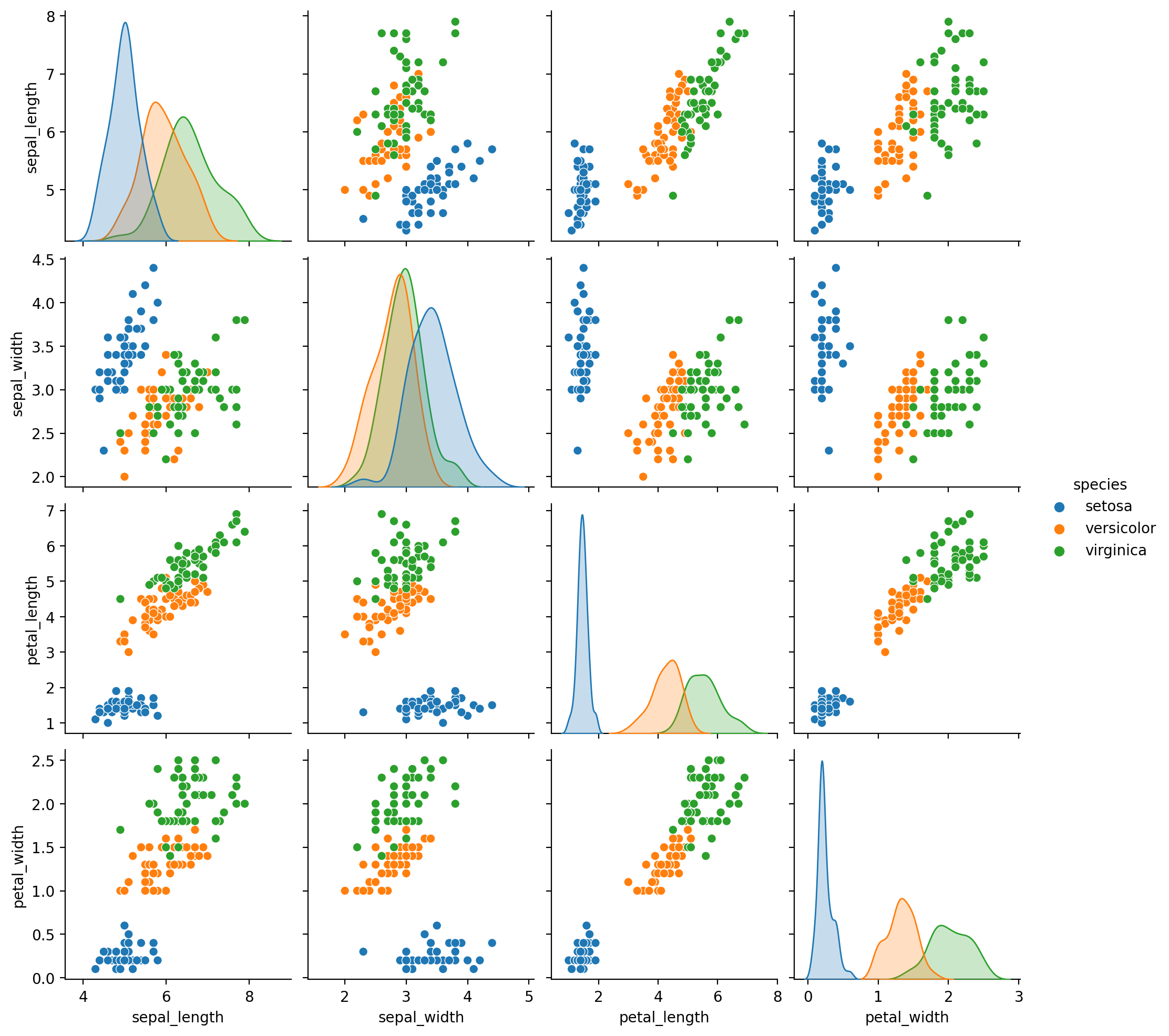
I find that I learn more efficiently by doing. So there will be some practical examples mixed in these posts. For my first practical example I’ll use the classic, Fisher’s Iris data set, which he introduced in 1936! It is a rather small dataset consisting of 3 different flower types and 50 examples of each flower type. The 3 classes are Iris-Setosa, Iris-Versicolour, Iris-Virginica. And the 4 features are sepal length, sepal width, petal length, petal width all in cm.

Probability theory
In order to classify an unknown flower $x$ as class $y_i$ (setosa, versicolour, virginica) we need to know what the probability is that $x$ is of class $y_i$. This means we need to know all the:
Once we have all the posterior probabilities we can predict (classify) the species of a given flower $x$ by maximizing the posterior probability. The same principle holds for a regression problem, where $y$ is continuous.
Bayes’ theorem
Class (conditional) distribution p(x|y): To find the distribution of objects within a class based on examples, we will have to estimate a PDF (probability density function). One way of doing this is via Parametric density estimation.
Class prior p(y): The class prior represent the probability that an object is of class $y_i$, regardless of what the value of the object is. Given you have a large enough and Unbiased sample space this should be easily attainable.
Data distribution p(x): The data distribution tells you what the probability is that an object has value $x$, regardless of it’s class. Once both the Class priors and the Class (conditional) distributions of a certain dataset have been found, the data distribution can be calculated by summing the class priors with the distributions.
Generative learning algorithms
Generative learning algorithms try to model the underlying Class conditional distribution of each class. This distribution can intuitively be thought of as the distribution of which samples of the corresponding class are generated from.
To make a prediction however you need the posterior probabilities, therefore Bayes’ theorem is used.
Discriminative learning algorithms
Discriminative algorithms model the posterior probabilities from training examples directly. It makes fewer assumptions on the distributions but depends heavily on the quality of the data.
Conclusion
I’ve shortly introduced the supervised machine learning and talked about the two distinct ways to tackle learning algorithms. In future posts I’ll go more in depth in certain algorithms and explain their advantages / disadvantages.