Gaussian Discriminative Analysis

2019-12-20

5 min read

If I sample many many apples from a basket of independent identically distributed (i.i.d.) randomly sized appels, the distribution of the size of my apples will converge towards the Gaussian distribution. This is what Laplace came up with in 1812, in his “Analytic Theory of Probability”. Although Carl Friedrich Gauss 3 years before that already introduced the function and worked out the least squares approximation to estimate the ’true’ (mean) value from a bunch of i.i.d. measurements (very usefull in statistics / confidence calculations).

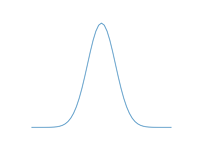
1D Gaussian

\[\begin{aligned} \mathcal{N}(\mu, \sigma^{2}) = \dfrac{1}{\sigma \sqrt{2\pi}} \exp{(-\dfrac{1}{2} ( \dfrac{x-\mu}{\sigma})^{2})} \end{aligned}\]

Now lets get back to machine learning …. We can use a the Gaussian distribution to model the PDF of features. And if you remember, we can use Bayes’ theorom to caculate the posterior distribution from the PDF and so we can make a prediction algorithm!

Parametric Density Estimation: To get an idea of the underlying distribution of the features we try to estimate this distribution based on a formula with parameters. Most commenly used formula for parametric density estimation is the Gaussian distribution:

Quadratic discriminate analysis

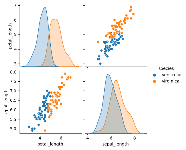
Lets say we only have two features of Fishers’ Iris dataset available, for example petal length and sepal length and we are only dealing with two species instead of three (making the example as easy as possible to visualize it).

The Quadratic discriminate analysis is an algorithm that predicts the species based on the two features. This does require the multivariate version of the Gaussian so let’s have a look:

Multivariate Gaussian

\[\begin{aligned} \mathcal{N}(\mu, \Sigma) = \dfrac{1}{(2\pi)^{n/2} |\Sigma^{1/2}| } \exp{(-\dfrac{1}{2} (x-\mu)^{T} \Sigma^{-1} (x-\mu) )} \end{aligned}\]

In binary (two species) QDA the classification is based on the discriminant:

\[\begin{aligned} f(x) = \text{log} \ p(y_1 | x) - \text{ log } \ p(y_2 | x) \end{aligned}\]

A positive discriminant means the posterior probability of class 1 is higher and thus we classify $x$ as class 1. The log of the posterior probabilities is taken because this yields a simpler (more efficient) equation. This is possible because log is a monotonically increasing function, which means that the relations of order are unchanged. The $max_i$ $p(y_i|x)$ will also be the $max_i$ log $p(y_i|x)$. From the log of the posterior probability follows:

\[\begin{aligned} p(y_i|x) &= \dfrac{p(x|y_i)p(y_i)}{p(x)} \\ \log{p(y_i|x)} &= \log{p(x|y_i)} + \log{p(y_i)} - \log{p(x)} \\ &= -\dfrac{p}{2}\log{2\pi} -\dfrac{1}{2}\log{\det{\Sigma_i}} - \dfrac{1}{2}(x-\mu_i)^T\Sigma_i^{-1}(x-\mu_i) \\ &+ \log{p(y_i)} - \log{p(x)} \\ \end{aligned}\]

Removing all non-class dependent constants yields:

\[\begin{aligned} \log{p(y_i|x)} &= -\dfrac{1}{2}\log{\det{\Sigma_i}} - \dfrac{1}{2}(x-\mu_i)^T\Sigma_i^{-1}(x-\mu_i) + \log{p(y_i)} \end{aligned}\]

Plugging the result into the discriminant equation yields:

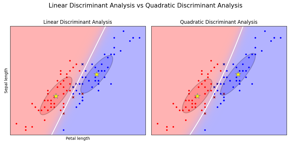
\[\begin{aligned} f(x) &= \log{p(y_1|x)} - \log{p(y_2|x)} \\ f(x) &= x^T W x + w^T x + w_0 \\ W &= \dfrac{1}{2} (\Sigma_2^{-1} - \Sigma_1^{-1}) \\ w &= \mu_1^T\Sigma_1^{-1} - \mu_2^T\Sigma_2^{-1} \\ w_0 &= -\dfrac{1}{2}\log{\det{\Sigma_1}} - \dfrac{1}{2}\mu_1^T\Sigma_1^{-1}\mu_1 + \log{p(y_1)} \\ &+ \dfrac{1}{2}\log{\det{\Sigma_2}} + \dfrac{1}{2}\mu_2^T\Sigma_2^{-1}\mu_2 - \log{p(y_2)} \\ \end{aligned}\]

This is a quadratic equation modeling the decision boundary for a two class classification problem. The final class prediction or hypothesis $h(x)$ is then given by the following bernouilli distribution.

Linear discriminate analysis

Given the assumption that the covariance matrices of both classes are equal $(\Sigma_1 == \Sigma_2)$, the decision boundary becomes linear:

\[\begin{aligned} f(x) &= w^T x + w_0 \\ w &= \hat{\Sigma}^{-1} (\hat{\mu}_2 - \hat{\mu}_1) \\ w_0 &= \dfrac{1}{2} \hat{\mu}_2^T \hat{\Sigma}^{-1} \hat{\mu}_2 - \dfrac{1}{2} \hat{\mu}_1^T \hat{\Sigma}^{-1} \hat{\mu}_1 + \log{\dfrac{p(y_1)}{p(y_2)}} \\ \end{aligned}\]

Also called Fisher’s Linear Discriminate analysis.

Fisher Iris Example

Code for this was taken from: https://scikit-learn.org/stable/auto_examples/classification/plot_lda_qda.html#sphx-glr-auto-examples-classification-plot-lda-qda-py

Side Note: LDA as a dimensionality reduction technique

In Fisher’s article he observes that at the decision boundary (discriminant = 0), the ratio of between and within class variance is:

\[\begin{aligned} \Phi = \dfrac{\text{variance between}}{\text{variance within}} = \dfrac{[\omega \mu_1 - \omega \mu_0]^2}{\omega^T \Sigma_1 \omega + \omega^T \Sigma_0 \omega} \end{aligned}\]

Here $\omega$ is a unit vector in a certain direction. He furthermore obeserves that this ratio is maximal for, $\omega$ as in LDA:

\[\begin{aligned} \omega &= \hat{\Sigma}^{-1} (\hat{\mu}_2 - \hat{\mu}_1) \\ \end{aligned}\]

The simple interpretation of this is that, the dicision boundary has a slope which is equal to the direction of maximum $\Phi$.

The use LDA as a dimensionality reduction technique all you have to do is map the data onto the first $k$ principal axes of the $\Phi$. (Later on we will have a look at other similar dimensionality reduction technique such as PCA)

Conclusion

We’ve looked at two variants of parametric generative algorithms to predict flower species from petal / sepal lengths. For our small test example lda and qda were quite alright, but it’s good to know what the limitations are.

QDA assumptions/limitations:

It assumes the PDF of the class conditional distributions can be modelled by a Gaussian.
The decision boundary generated by QDA is quadratic.
It uses Bayes’ rule to get from class conditional distributions to posterior distribution and to achieve this the class priors are used. So for datasets with imbalanced example count per class this can induce a bias for a specific class with a higher example count.

LDA assumptions/limitations:

Like Qda, it assumes the PDF of the class conditional distributions can be modelled by a Gaussian, but it goes one step further by assuming that all classes share a PDF with the same covariance matrix.
The decision boundary generated by LDA is linear.
It uses Bayes’ rule to get from class conditional distributions to posterior distribution and to achieve this the class priors are used. So for datasets with imbalanced example count per class this can induce a bias for a specific class with a higher example count.