Logistic Regression

2020-01-15

3 min read

Logistic regression

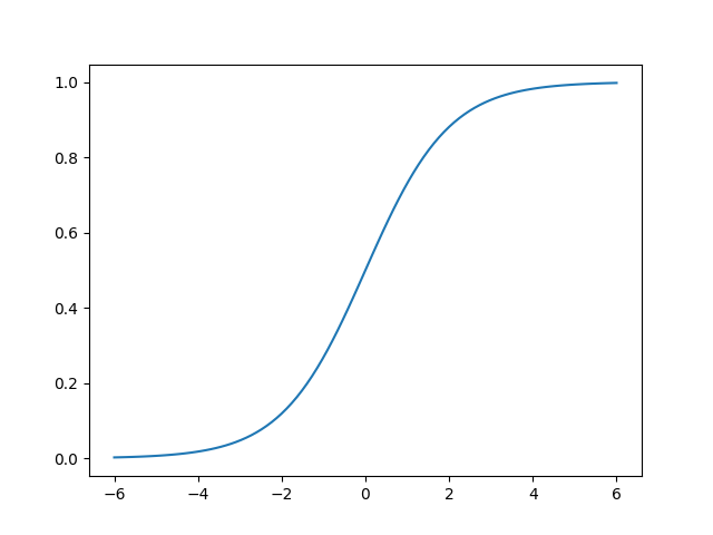
Logistic regression unlike linear regression is well suited for classification type problems. The difference lies in the way data is fitted, instead of a linear (hyper)plane it is fitted using the following exponential function (also known as the sigmoid function):

\[\begin{aligned} h_{\theta}(x) = \dfrac{1}{1 + \exp{(-\theta^Tx)}} \end{aligned}\]

This function has the nice property that, its output is bound between zero and one. This is a usefull property when trying to model the (posterior) probability of something. In a two class classification problem, where the output is either a one or a zero, a bounded function intuitively also makes more sence.

The derivative of $h_{\theta}(x)$ is going to be usefull later on, for gradient descend.

\[\begin{aligned} \dfrac{\delta h_{\theta}(x)}{\delta \theta} &= \dfrac{1}{(1 + \exp{(-\theta^Tx)})^2} \cdot -x \exp{(-\theta^Tx)} \\ &= \dfrac{1}{(1 + \exp{(-\theta^Tx)})} \cdot -x \dfrac{\exp{(-\theta^Tx)}}{(1 + \exp{(-\theta^Tx)})} \\ &= \dfrac{1}{1 + \exp{(-\theta^Tx)}} \cdot -x ( \dfrac{1 + \exp{(-\theta^Tx)}}{1 + \exp{(-\theta^Tx)}} - \dfrac{1}{1 + \exp{(-\theta^Tx)}} ) \\ &= x h_{\theta}(x) (1 - h_{\theta}(x)) \end{aligned}\]

Cost function

In a two class binary classification example the posterior probability of the logistic regression function is modeled using the bernoulli distribution:

\[\begin{aligned} p(y_i|x;\theta) &= \begin{cases} h_{ \theta }(x) &: i=1 \\ 1-h_{ \theta }(x) &: i=0 \end{cases} \\ p(y_i|x;\theta) &= h_{\theta}(x)^{y_i}(1-h_{ \theta }(x))^{1-y_i} \end{aligned}\]

The cost function for the logistic regression method will again be formulated based on the likelihood of the data given the parameter $\theta$. The Likelihood is defined as the cumulitive probability of the correct class for all given training objects. The likelihood of a dataset (assuming samples were drawn independently):

\[\begin{aligned} L(\theta) &= p(y|x;\theta) \\ &= \prod_{i=1}^n p(y^{(i)} | x^{(i)}) \\ &= \prod_{i=1}^n h_{\theta}(x^{(i)})^{y^{(i)}} (1-h_{\theta}(x^{(i)}))^{1-y^{(i)}} \end{aligned}\]

To use this likelihood in our gradient descend alogrithm we will transform it in the following way. Because the gradient descend algorithm optimizes for finding the minimum cost, we will have to take the negative likelihood. Taking the log of the likelihood will make computations a lot easier without affecting the outcome. Another reason for taking the log of the likelihood is to prevent the likelihood from converging towards zero very quickly as the dataset volume increases.

\[\begin{aligned} J(\theta) &= - \text{log} \ (L(\theta)) \\ &= \sum_{i=1}^n -y^{(i)} \text{log} \ ( h_{\theta}(x^{(i)}) ) + (y^{(i)}-1) \text{log} \ (1 - h_{\theta}(x^{(i)})) \end{aligned}\]

Gradient descend

The update rule for our stochastic gradient descend (one training example) algorithm will look as follows:

\[\begin{aligned} \theta :&= \theta + \alpha \cdot \dfrac{\delta J(\theta)}{\delta \theta} \\ &= \theta - \alpha \cdot \left( -y \dfrac{1}{h_{\theta}(x)} - (y-1) \dfrac{1}{1 - h_{\theta}(x)} \right) \dfrac{\delta h_{\theta}(x)}{\delta \theta} \\ &= \theta - \alpha \cdot \left( -y \dfrac{1}{h_{\theta}(x)} - (y-1) \dfrac{1}{1 - h_{\theta}(x)} \right) x h_{\theta}(x) (1 - h_{\theta}(x)) \\ &= \theta - \alpha \cdot x \cdot ( \ (1-y)h_{\theta}(x) - y(1-h_{\theta}(x)) \ ) \\ &= \theta + \alpha (y - h_{\theta}(x)) x_j \end{aligned}\]